How It Works

What this model is, and is not

It is a modified point-mass model: the bullet is treated as a point with mass and a drag profile, stepped through time rather than solved in one formula. Spin drift and crosswind jump are empirical add-ons, not full orientation physics. Use it to compare loads and practice reading wind.

It is not a promise of what your rifle will do on a given day. Coriolis and Eötvös drift, powder-temperature effects on muzzle velocity, bore and rifle imperfections, and error in your wind, range, and atmosphere inputs are outside the model. Enter a chronographed muzzle velocity and treat the numbers as an estimate.

How a trajectory is computed

A flying bullet is pushed by three things: gravity pulling it down, aerodynamic drag opposing its motion through the air, and, because it is spinning, small gyroscopic effects sideways and vertically. The engine sums these into an acceleration and steps the bullet forward through time. The bullet's state is its position \(\mathbf{x}\) and velocity \(\mathbf{v}\):

\[ \frac{d\mathbf{x}}{dt} = \mathbf{v}, \qquad \frac{d\mathbf{v}}{dt} = \mathbf{a} = \mathbf{a}_{\text{drag}} + \mathbf{g} + \mathbf{a}_{\text{spin}}, \qquad \mathbf{g} = (0,\,-9.80665,\,0)\ \tfrac{\text{m}}{\text{s}^2} \]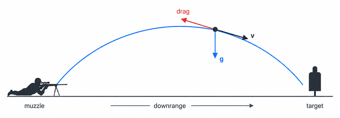

This is a 3-DOF translational model: position and velocity are integrated, the bullet's orientation is not. Spin drift enters as an extra acceleration each step; crosswind jump enters as a vertical velocity kick when crosswind changes. Both apply only when spin effects are enabled (see Spin corrections). That is what "modified" point-mass means.

Drag and ballistic coefficient

Drag is the main force slowing the bullet, and it changes sharply with speed, especially near the sound barrier. Rather than one drag number, the engine pairs a standard drag function (a reference curve for a typical bullet shape) with your ballistic coefficient (BC), which says how your bullet compares to that reference. A higher BC means the bullet holds speed better, so less drop and less wind drift.

• G1 is a flat-based reference shape, a good match for older flat-based bullets. It fits modern boat-tail bullets poorly, so no single G1 BC holds across the speed range: the value needed to match the real drag changes with velocity, which is why G1 BCs are often published in velocity bands.
• G7 is a boat-tail reference shape that matches modern long-range boat-tail bullets, giving a more constant BC across the supersonic range. G7 is the engine default.

Each drag function is the standard drag coefficient curve \(C_d\) versus Mach number for its reference shape, the tabulated McCoy / JBM G1 and G7 data, which the engine linearly interpolates. Every step it forms the bullet's Mach number from its air-relative speed and the local speed of sound \(a_{\text{snd}}\), looks up \(C_d\), and scales by air density and the BC:

\[ M = \frac{v_r}{a_{\text{snd}}}, \qquad \mathbf{a}_{\text{drag}} = -\,\frac{C_d(M)\,v_r^{2}}{k\,\text{BC}}\cdot\frac{\rho}{\rho_0}\;\hat{\mathbf{v}}_r, \qquad v_r = \lVert \mathbf{v}-\mathbf{w}\rVert \]

Here \(\mathbf{w}\) is the local wind, \(\rho\) the current air density, \(\rho_0 = 1.225\ \text{kg/m}^3\) the reference density, and \(k\) a fixed constant that folds in the standard projectile's reference size (a 1 lb, 1 inch bullet). Because drag is keyed to Mach, the steep transonic drag rise sits at a different airspeed depending on conditions: a warmer day raises the speed of sound, so the bullet meets that spike at a higher fps than on a cold one. Within this point-mass model, once the drag function and BC are fixed, bullet diameter and weight do not separately affect drag; they re-enter later through the spin and stability corrections, where mass, caliber and length matter.

You can see this directly below. Enter a bullet's G1 and G7 BC and the chart draws its actual deceleration under each model (the standard drag curve divided by the BC you give). For a properly matched pair (the same bullet's published G1 and G7 numbers) the two curves nearly coincide over the supersonic band the BCs were fit for, then split apart through the transonic region and out at the speed extremes, where the single-number G1 fit can no longer track the boat-tail's true drag. That gap is why a single G1 number can't follow a boat-tail everywhere: staying accurate with the G1 model takes velocity-banded BCs or a published drag curve, whereas a single G7 number stays far closer across that range. Neither is exact, since a real bullet only approximates either reference shape, but G7 fits modern boat-tails much better, and the bullet's own measured drag curve is closer still.

Show Deceleration Drag coefficient G1 BC G7 BC Log y

Stepping the bullet through time

Because drag depends on speed and speed keeps changing, there is no closed-form path; it is computed step by step. The engine uses a second-order Runge–Kutta (RK2) midpoint step. A naive step trusts the slope at the start and overshoots; RK2 instead samples the slope at the middle of the step and uses that for the whole step. That costs a second acceleration evaluation per step (two instead of one), but it is accurate enough to allow much larger steps for the same error, so it is a good trade overall.

\[ \mathbf{v}_{1/2} = \mathbf{v}_0 + \tfrac{1}{2}\mathbf{a}_0\,\Delta t, \qquad \mathbf{x}_{1/2} = \mathbf{x}_0 + \tfrac{1}{2}\mathbf{v}_{1/2}\,\Delta t, \qquad \mathbf{a}_{1/2} = \mathbf{a}\!\left(\mathbf{x}_{1/2},\,\mathbf{v}_{1/2},\,t_0+\tfrac{1}{2}\Delta t\right) \] \[ \boxed{\;\mathbf{v}_{1} = \mathbf{v}_0 + \mathbf{a}_{1/2}\,\Delta t, \qquad \mathbf{x}_{1} = \mathbf{x}_0 + \mathbf{v}_{1/2}\,\Delta t\;} \]

The simulation marches until the bullet passes the requested distance (or a time cap); values at exact distances are interpolated between the two stored points that bracket them.

Air density and atmosphere

Drag scales with air density, which depends on temperature, altitude and humidity, so the same bullet drops and drifts less in thin mountain air than in cold, dense sea-level air. You enter temperature, altitude and humidity; pressure is derived from the altitude. Density comes from the ideal gas law with a humidity correction (moist air is slightly less dense, the \(0.378\,e\) term):

\[ \rho = \frac{P - 0.378\,e}{R_{\text{air}}\,T}, \qquad R_{\text{air}} \approx 287.05\ \tfrac{\text{J}}{\text{kg}\cdot\text{K}}, \qquad e = \text{RH}\cdot 611.2\,\exp\!\left(\frac{17.67\,T_c}{T_c + 243.5}\right) \]

Pressure follows the International Standard Atmosphere power law from altitude \(h\):

\[ P = P_0\left(1 + \frac{L\,h}{T_0}\right)^{-g/(R_{\text{air}} L)}, \qquad P_0 = 101325\ \text{Pa},\; T_0 = 288.15\ \text{K},\; L = -0.0065\ \text{K/m} \]

In the integrator, density scales drag through the ratio \(\rho/\rho_0\). The Miller stability factor is corrected separately with muzzle temperature and pressure (see Spin corrections), so a cold, high-pressure day slows the bullet more and can also lower gyroscopic stability.

How wind enters the model

Drag acts on the bullet's velocity relative to the air. So wind enters by subtracting it from the bullet's velocity before computing drag: the \(\mathbf{v} - \mathbf{w}\) you already saw in the drag equation. A crosswind tilts the drag vector slightly downwind, and integrated over the flight that becomes lateral drift. There is no separate "wind drift formula"; drift, the small range effect of a head or tail wind, and the interaction of wind with a slowing bullet are all handled by the same integration path.

The model never tracks which way the bullet is pointing: ordinary wind drift falls out of air-relative drag alone. The two effects that do depend on the bullet's orientation, spin drift and the crosswind's vertical jump, are handled separately under Spin corrections.

Calculator-style tools use a single uniform wind across the flight. The simulators sample a full wind field that varies with range, crossrange and time, so the bullet flies through different wind at every point; that field is described below.

Spin corrections

Rifling spins the bullet so it stays pointed forward. Its center of pressure sits ahead of its center of mass, so left to itself the bullet would tumble; the spin is what holds it nose-first.

A spinning bullet also behaves like a gyroscope. Its spin is captured by the angular-momentum vector \(\mathbf{L}\), which lies along the bullet's axis: by the right-hand rule, curl your right fingers the way the bullet is turning and your thumb points along \(\mathbf{L}\). A right-hand twist therefore points \(\mathbf{L}\) forward, downrange; a left-hand twist points it back toward the shooter. The gyroscopic part is that a sideways force on a spinning body is answered a quarter-turn away (a spinning top leans and circles instead of toppling over), and that 90° response is the source of two small deflections that grow with range, spin drift and crosswind jump.

Both are genuine gyroscopic effects, but the engine does not track the bullet's orientation to find them. Instead it uses empirical formulas from Bryan Litz (Applied Ballistics), physics-motivated curves with constants fitted to measured data, adapted to run inside the step-by-step integration.

Gyroscopic stability (Miller)

A stability factor \(S_g\) measures the spin margin, starting from the Miller twist rule and corrected to the actual velocity and air conditions:

\[ S_{g,0} = \frac{30\,m}{t^{2}\,d^{3}\,l\,(1+l^{2})}, \qquad S_g = S_{g,0}\left(\frac{V}{2800}\right)^{1/3}\frac{T_R}{519}\cdot\frac{29.92}{P_{\text{inHg}}} \]

with \(m\) in grains, \(d\) in inches, \(l = L/d\) the length in calibers, \(t\) the twist in calibers per turn, \(V\) in fps, \(T_R\) in °Rankine and \(P_{\text{inHg}}\) in inches of mercury. As a rule of thumb \(S_g > 1.5\) is stable. The Miller rule assumes roughly uniform bullet density; the engine uses the standard form only.

Spin drift

As the bullet flies, gravity steadily bends its path downward. The spin makes the bullet's axis gyroscopically stiff, so the nose cannot quite follow that curve: it lags, and rides slightly above the path. The oncoming air then meets the nose at a small angle, and the same quarter-turn response leans that to one side: the nose takes up a small sideways lean, its yaw of repose. Because the nose points a little to the side throughout the flight, the bullet is continually nudged that way, and the drift accumulates with range, to the right for a right-hand twist.

Litz gives an empirical fit for that sideways displacement as a function of time of flight:

\[ \text{SD}(t) = 1.25\,(S_g + 1.2)\;t^{1.83}\quad[\text{inches}] \]

A point-mass integrator cannot simply add a displacement on top of its path, so the engine differentiates the law twice and injects it as a sideways acceleration, letting the same RK2 step reproduce the curve:

\[ a_{\text{spin}}(t) = \frac{d^{2}\text{SD}}{dt^{2}} = 1.83\cdot 0.83\,C\,t^{-0.17}, \qquad C = 1.25\,(S_g + 1.2) \]

Crosswind aerodynamic jump

A horizontal crosswind shifts the shot vertically, the crosswind jump, through the same gyroscopic response. The wind pushes on the bullet's center of pressure, which sits ahead of its center of mass, and that yaws the nose to the side. But a gyroscope answers a sideways push a quarter-turn away, so most of that yaw is turned into the vertical: the shot lands high or low even though the wind is purely horizontal. This is not the same as wind drift. Drift builds up over the whole flight, while the jump is a single angular kick, delivered as the bullet first meets the wind (at the muzzle for a steady crosswind). Apply a crosswind in the demo below to see it.

Litz gives the size as a sensitivity (roughly 0.3–0.5 MOA per 10 mph at 1000 yd). For a right-hand twist, wind from the right makes the shot land high and wind from the left low; a left-hand twist reverses it:

\[ \text{sens} = 0.01\,S_g - 0.0024\,\frac{L}{d} + 0.032 \quad[\text{MOA per mph}] \]

With that understood: each step, the engine compares the crosswind the bullet sees to the previous step and fires an impulse proportional to the change \(\Delta w_\perp\) (in mph), so a constant wind fires its whole jump at the muzzle while a gust met downrange fires there. That change sets a small jump angle \(\Delta\theta = \text{sens}\cdot\Delta w_\perp\), applied as a kick to the bullet's vertical velocity before the RK2 step, where \(\text{hand}=\pm1\) sets the sign from the twist direction:

\[ \Delta v_y = -\,V\,\Delta\theta\cdot \text{hand} \]

This assumes the jump is effectively instantaneous, that the muzzle sensitivity still applies downrange, and that successive wind changes add up linearly, all approximations.

See it for yourself

The bullet below spins about its long axis, the angular-momentum vector L, slowed right down so you can read the rifling turning. Use the Effect buttons to switch between the crosswind jump just described and spin drift, its gravity-driven cousin: gravity bends the path, the spinning nose lags above it, and the same quarter-turn response leans that into a steady sideways drift. Flip the twist to reverse the directions (and the rifling), and drag to orbit the view.

Effect Crosswind jump Spin drift

Twist Right-hand Left-hand

Crosswind From left Off From right

Axes & vectors

Smooth noise: the building block

The wind field and mirage both use simplex noise (Ken Perlin's gradient noise), but separate instances: each wind layer curls its own potential \(\psi\), while mirage shaders warp the scope with their own samples (Steel mirage does not read the curl field at all). Unlike a table of independent random numbers, simplex noise is continuous: nearby points return nearby values, with no grid and no sudden jumps, and it is cheap to evaluate and to differentiate.

It works by pinning a random direction (a gradient) at each point of a coarse lattice and smoothly blending their pull: the value climbs toward some neighbors and dips toward others, giving the rolling hills and valleys below. It also varies on a single scale, changing gradually from place to place with no fine jitter, which is what lets it read as a coherent gust pattern rather than random static. One smooth number comes out at every point, and the wind field calls that number the potential \(\psi\). The simulators sample it in three or four dimensions (downrange, crossrange, and time for wind; F-Class mirage adds another spatial axis), so the pattern evolves smoothly rather than flickering frame to frame.

The wind generator

The simulators do not blow one constant wind down the range; they generate a wind field that swirls, varies along the range, and evolves over time. You can explore it in the Wind Generator tool.

From \(\psi\) to wind

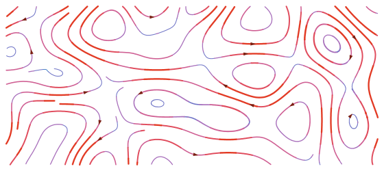
Simplex noise gives a smooth height \(\psi\) over the range. Horizontal wind is the curl of \(\psi\) in the downrange/crossrange plane:

\[ \mathbf{w}_{\text{raw}} = \left(\frac{\partial\psi}{\partial y},\,-\frac{\partial\psi}{\partial x}\right) \]

Wind follows the contour lines of \(\psi\), circling its highs and lows rather than running up or down the noise surface. The field is non-diverging: because \(\mathbf{w}_{\text{raw}}\) is a curl, \(\nabla\cdot\mathbf{w}_{\text{raw}} = 0\), so streamlines form closed loops instead of starting or stopping in place. Speed is greatest where \(\psi\) changes fastest.

Post-processing: from curl to the wind you feel

The bullet and mirage sample the post-processed field, not \(\mathbf{w}_{\text{raw}}\). The curl supplies eddy structure and direction; the pipeline below sets how strong each layer blows, how calm or gusty it feels, and how layers add up before they are summed. It reshapes speed along the curl direction only; it never rotates the flow. The steps, in order:

1. Curl. Sample \(\psi\) with 3D simplex noise (downrange, crossrange, and time) and estimate its slope with small finite differences. Each layer uses its own stretch along downrange and crossrange (a 10,000-yard layer vs a 100-yard layer), so the same noise feature can represent a broad shift or a tight gust; those stretches are undone when converting the curl back to real range coordinates. The result is a horizontal vector only (crossrange and downrange; no vertical wind from this step).
2. Polar split. Convert the curl vector to magnitude and direction. All later steps rescale the speed along that fixed direction; they never rotate the flow or inject unrelated vectors.
3. RMS normalization. Divide the magnitude by a constant RMS estimated on the first tick of the wind clock from ~1000 random samples of that component. This makes each layer's energy stable before the preset's strength knob is applied.
4. Exponent. Raise the normalized magnitude to a power \(p\). Values \(p < 1\) even out the layer toward a steadier average; \(p > 1\) make it mostly calm with occasional surges. Most presets keep \(p \le 1\); the Turbulent preset uses \(p = 1.2\) on its finest layer.
5. Strength scale. Multiply by the component strength. This sets the layer's nominal speed.
6. Sigmoid gate (optional). Some layers pass the magnitude through a logistic gate so the component stays quiet below a threshold and switches on above it, producing distinct gust events rather than always-on turbulence.
7. Clip. Cap the magnitude at \(2S\) (twice the component strength) so a single sample cannot run away.
8. Sum. Rebuild a Cartesian vector from the final magnitude and the saved direction, map into BTK coordinates \((x=\) crossrange, \(y=0\), \(z=-\) downrange), and add all components at the query point.

Constant-factor steps (RMS normalization and strength scale) keep the field non-diverging. Nonlinear steps (exponent when \(p \ne 1\), sigmoid gate, and clip) break that on purpose: they trade the non-diverging guarantee for calmer averages, sharper gusts, and hard speed limits. Directions still come from the curl throughout, so the finished field remains visibly eddy-like.

Layering, presets, and advection

Several components stack: a broad slow base wind, a medium gusting layer, and fine turbulence, each with its own spatial scales (downrange and crossrange), temporal scale, strength, exponent, and optional gate. Named presets (Zero, Dead, Calm, Moderate, Strong, Extra Strong, Switchy, Turbulent, Gusty, and Shear) are different recipes of those layers. The Moderate preset, for example:

Layer	Strength	Scale (down × cross)	Time	Exponent	Gate	Role
Base	3 mph	10000 × 10000 yd	10 min	0.5	off	Slow overall condition
Gust	3 mph	1000 × 1000 yd	1 min	0.75	1.0× strength	Gusts & switches
Turbulence	1 mph	100 × 100 yd	0.5 min	1.0	off	Fine jitter

On top of that, the whole pattern advects: the whole pattern slides downrange as one instead of just churning in place, carried by the mean wind. This loosely follows Taylor's frozen-turbulence hypothesis, the idea that over short times the eddies are swept past mostly intact by the mean flow rather than reshaping where they sit. Each frame the generator estimates that mean wind by averaging the composite field at several random points across the range (a rough proxy for the prevailing flow), smooths it with an exponential moving average, scales it by the advection multiplier \(m\), and integrates it into a global offset \(\mathbf{o}\) that is subtracted from the sampling coordinates when the curl is evaluated. Eddies therefore travel downrange with the prevailing flow rather than merely morphing in place.

\[ \mathbf{U} \leftarrow (1-\alpha)\,\mathbf{U} + \alpha\,m\,\langle\mathbf{w}\rangle, \qquad \mathbf{o} \mathrel{+}= \mathbf{U}\,\Delta t \]

The advection multiplier \(m\) is greater than 1, with a rough physical rationale: wind generally increases with height, and a turbulent eddy is a tall structure, so it may be carried partly by the faster wind above the deck and drift downrange somewhat faster than the wind sampled near the ground. The preset values are tuned by hand so the streaming reads clearly; treat the multiplier as a tuning knob with a plausible physical rationale, not a measured quantity.

Why not simulate the air for real? True computational fluid dynamics would solve the Navier–Stokes equations on a fine grid, far too expensive to run live in a browser. It would not buy much realism here anyway: a real solve still needs boundary conditions and gusty inflow that are effectively unknown, so the important randomness has to be invented either way. Curl noise plus the shaping pipeline above gives coherent, plausible, cheap eddies directly.

Mirage and scope optics

What mirage is: on a warm day the ground heats the air just above it, and that warm air rises in shifting cells. Warm and cool air bend light by different amounts, so when you look through a scope at a distant target the image wavers and "boils." In wind the boil leans, or "runs," in the wind's direction and flattens as the wind builds, so reading it is one of the main ways shooters judge the wind downrange.

How it is drawn: both simulators fake this with a screen-space post-process, not a ray-traced heat shimmer. The 3D scene is rendered to an off-screen buffer first; a full-screen shader then nudges each pixel by simplex noise advected by the same post-processed wind field the bullet integrates through. It is a visual approximation that preserves the cues a shooter reads (which way the boil runs and how strong it is), not a simulation of light actually bending.

Mirage fades as wind builds and is gone by about 15 mph in both sims, keyed to wind speed. They differ in how many depth layers they use, how they sample the wind field, and whether a separate lens blur runs as well. The pipelines below are the actual render order.

The scope camera and projection

Each scope is a full 3D render through its own perspective camera, not a crop of the main view. The camera sits at the shooter's eye and points where the shooter is aiming: its look direction is set by the current yaw (horizontal) and pitch (vertical). Recoil is applied to that same aim, so on the shot the camera kicks. The reticle is a fixed overlay, so it holds its place at the center of the frame, but its point of aim moves with the camera, so the target jumps out from under it, just as it does through a real scope.

Zoom is the field of view. Magnification runs inversely with FOV, so raising the power narrows the FOV; the new FOV is written to the camera and its projection matrix is rebuilt. Near and far clip planes bound the rendered depth (in Steel, roughly 30 to 2500 yards), and a tight far plane also sharpens the depth buffer that the blur and mirage sample. The camera's aspect ratio comes from the scope's render target.

The reticle is built in angular units and tied to that projection. A first-focal-plane (FFP) reticle scales with zoom so each mark keeps its true angle: Steel scales the reticle by \(\tan(\theta_\text{init}/2)\,/\,\tan(\theta_\text{cur}/2)\), where \(\theta\) is the field of view at the initial and current zoom. F-Class can run either an FFP reticle or a second-focal-plane (SFP) reticle, which holds a fixed on-screen size and is calibrated only at the initial zoom.

Depth of field: the lens model

The Steel scope's focus blur is an angular depth-of-field model, not a fixed screen blur. For each pixel the depth buffer gives the distance \(d\) to whatever is drawn there, and the focus distance \(d_f\) is the scope's current focus setting. The blur is computed as an angle:

\[ \theta = k\,\frac{D}{d_f}\,\left|\frac{d - d_f}{d}\right| \]

\(D\) is the objective diameter (a 56 mm aperture), so the aperture-over-focus term sets the size of the defocus cone, and the last factor is how far the pixel sits off the focal plane, zero at the focus distance and growing on either side of it. A tuning constant \(k\) scales the overall strength, and the angle is capped at about 1 mrad so nothing smears too far. Computing the blur as an angle and only then converting it to a pixel radius (through the camera's FOV) keeps it consistent across window size and zoom: the same defocus reads as the same blur whatever the resolution.

That radius drives a separable Gaussian blur, two passes (horizontal then vertical) with Gaussian weights and a sample count that grows with the radius but is capped at 16 per side; a pixel within about a tenth of a pixel of sharp is passed through untouched. Because the amount is driven by each pixel's own depth, only the out-of-focus range softens while whatever sits at the focus distance stays crisp, the shallow depth of field of a high-magnification optic. F-Class runs no blur pass at all.

F-Class Sim: scene, then mirage

1. Scene pass. Render the range through the scope's camera into an intermediate texture. The same path serves the rifle scope, which carries the reticle, and the spotting scope, which does not.
2. Wind sampling. Cast the scope's center ray into the range bounding box. Each of three atmospheric slabs along the line of sight picks a random point in its depth band, samples the wind generator there, and smooths the result with an exponential moving average. Each slab also takes a world scale equal to the viewport's world width at its depth, which grows with distance: the near slab spans a narrow slice of the scene, so a fixed-size patch of disturbed air fills much of the frame and reads as a large soft feature, while the far slab spans a wide slice, so the same patch reads as small and sharp.
3. Mirage pass. A full-screen shader sums one 4D simplex-noise sample per slab (three spatial axes plus time), advected by that slab's smoothed wind (crosswind shifts the pattern sideways, vertical wind and a constant heat rise shift it up, headwind churns the downrange axis slowly). The layers add into a vertical UV offset, and the scene texture is resampled at the warped coordinates. A faint cool tint, mixed in proportion to the local distortion, and an elevation falloff (mirage full when the sight grazes the deck, tapering off into the sky above the target) finish the look. Zoom scales intensity, capped so extreme magnification cannot sample absurdly far off-pixel.
4. Reticle composite. After the scene and mirage passes, the warped texture is shown on a quad in a shared composition scene, where the rifle scope's crosshair and dial readout are shader-drawn on top (the spotting scope has neither), so the reticle stays crisp and untouched by the mirage. Unlike Steel, this composite happens outside the scope's own render.

There is no depth-of-field blur in F-Class; the soft-near / crisp-far look comes only from the slab scaling. Mirage can be turned off entirely (preset None), which skips the mirage pass and draws the scene straight to the scope output.

Steel Sim: blur, then mirage

1. Scene + depth pass. Render the range into a buffer that carries a depth texture (distance per pixel).
2. Focus blur. A thin-lens model turns each pixel's depth and the scope's focal distance into a blur radius (growing with objective diameter and with distance from the focal plane). A separable Gaussian blur runs in two passes, horizontal then vertical, so only the focused range stays sharp.
3. Wind sampling. Because the shooter can look anywhere, the scope's focus distance sets how far downrange to sample the wind generator: seven points from 50% to 110% of that distance along the line of sight, averaged into one vector. Perpendicular wind and a constant heat rise advect the noise coordinates over time so the boil drifts and runs.
4. Mirage pass. A single-layer shader blends fast and slow 3D simplex noise (its own field, not the wind generator's curl). Each pixel's UV is shifted vertically by the noise amount, scaled by four attenuations: the per-pixel distance from the depth buffer (objects nearer than the focal distance barely boil, full strength at the focal distance and beyond), and three uniforms, magnification (none at a wide field of view), focal distance (longer reads as stronger), and total wind speed (fades to zero by about 15 mph). The same noise also darkens each pixel in proportion to its magnitude, a subtle smoke-like shading.
5. Reticle composite. The warped (and possibly blurred) scene is drawn into the final scope view; the reticle is overlaid on top so it stays crisp and unaffected by mirage or recoil kick on the underlying image.

In Steel a single optical-effects toggle governs both the focus blur and the mirage; with it off, both passes are skipped and the scene composites straight to the reticle.

Impact detection

A trajectory is a list of points in time and space. Detecting a hit means asking, for each short flight segment between two of those points, whether it pierced something. On the steel range that test is analytic: the segment is transformed into the target's own frame, where the plate lies flat at \(z=0\). The crossing parameter \(t\) is solved directly, and the crossing point is tested against the plate outline, a rectangle (\(|x|\le \tfrac{w}{2},\,|y|\le \tfrac{h}{2}\)) or an ellipse, expanded by the bullet radius so a round that just catches the edge still counts ("the line breaks the plate"):

\[ t = \frac{-\,z_{\text{start}}}{z_{\text{end}} - z_{\text{start}}}, \qquad \mathbf{p}_{\text{hit}} = \mathbf{p}_{\text{start}} + t\,(\mathbf{p}_{\text{end}} - \mathbf{p}_{\text{start}}) \]

The plate is treated as an infinitely thin face, not a 3D solid, so the geometry test reduces to a handful of dot products: all it needs is the contact point where the line pierces the face. That suits the physics, steel plates are thin, and the contact point is what fixes the splatter mark and the lever arm of the plate's reaction. How hard that reaction is driven depends on more than position, the bullet's speed and how square it strikes the plate, which the reactive-steel section below covers.

Culling with a range grid

The steel range can have many targets scattered downrange, and testing every segment of every bullet's path against every one of them would be wasteful. A shooting range is a long, mostly flat corridor, so the engine buckets the world into a flat grid laid over the ground, one axis crossrange, one axis downrange, with the vertical axis collapsed away. Each object is registered in the cells its footprint covers, and a flight segment is only ever tested against objects in the cells it passes through.

This is deliberately a uniform grid rather than the general 3D bounding-volume tree a game engine would normally reach for. The grid copes with moving targets cheaply, in two different ways. A target that wanders, like the walking boar, is just dropped from its old cells and re-added to its new ones as it goes, and only when it actually crosses a cell boundary. A swinging plate is handled more cheaply still: its footprint is registered once at a radius wide enough to enclose its entire swing arc, so it stays in the same cells and never has to be re-bucketed at all. A bounding-volume hierarchy, by contrast, would have to be refit constantly for exactly the objects that move the most. Collapsing the vertical axis costs nothing either, because a flat range barely uses it.

What a bullet can hit

Plates are not the only thing downrange. The detector also holds the reactive critter targets, the prairie dogs and the boar, and the solid scenery a round can actually strike: the berm behind everything, the frames the plates hang from, the wind-flag and windsock poles, and the yardage signs. Soft or distant detail is deliberately left out. The trees and the far terrain are simply not worth a collision, so a bullet passes straight through them. The flag and windsock cloth is skipped for a sharper reason: it is waved about by a vertex shader on the GPU, so its drawn shape never exists on the CPU to test against, and only the rigid pole is registered. Everything that is registered reduces to two geometry tests: steel plates use the fast analytic face test above, and the rest are triangle meshes tested with a standard ray-triangle intersection. Before either test runs, the segment is checked against the collider's axis-aligned bounding box with a quick slab test, and a segment that misses the box is dropped at once. That gate is what keeps the mesh path affordable: its real test brute-forces every triangle in the mesh, one after another, with no hierarchy inside the mesh to prune them, so the box check spares that whole sweep for all but the few colliders the segment actually reaches. A round that misses every target therefore still buries into the berm or clangs off a pole instead of flying on forever, and striking a piece of scenery scores as a miss.

The mesh path carries reactive game targets too, not just scenery, which is the other reason the grid's cheap updates matter. A prairie dog pops up and ducks back down, so its collider is switched on and off and only a raised one can be hit; the boar walks the range, so its collider, a simple box standing in for the animated model, is moved each frame to follow it. A hit on either throws a puff of red dust and drops the target, and its collider is then switched off so it no longer blocks later shots.

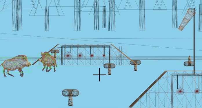
The Steel Sim does not integrate a bullet's whole path up front, the way the other apps do. Each frame it extends every in-flight bullet by one frame's worth of flight, a few integration steps, then hands the detector just that newly flown piece and asks for the first thing it crossed. Path and targets advance together, step for step. That lockstep is what lets a round hit a moving target at all: each newly flown piece is tested against the targets where they are at that instant, so a round can catch the walking boar or a plate still swinging from an earlier hit. The other apps integrate the whole path first because their targets never move.

Within a single check the trajectory's segments are in time order, so the earliest crossing is the one returned and the bullet strikes the first thing in its path rather than something farther along. The sim tracks every in-flight shot and runs this check for each one every frame. A confirmed hit on a plate writes a splatter into the plate's own paint texture (described below), puffs up metal-colored dust, plays a ping, and sets the plate swinging; steel deliberately takes no decal mark.

The simpler case: reading the trajectory at a distance

Everywhere outside the steel range there are no moving targets at various ranges, at most a single paper target at a fixed distance, so collision collapses into reading the integrated trajectory at that distance. The F-Class Sim still collides the bullet with its paper target, but because there is just one and its range is fixed, that reduces to reading the trajectory at exactly that distance, the one downrange plane that matters, in a single lookup. There is no segment crossing, no grid and no moving colliders to weigh: the bullet's crossrange and height at that distance, measured from the target center, give a 2D offset in the face of the target. Scoring is then purely radial, the distance from center compared against each ring radius and expanded by the bullet radius, so a round that just cuts a line takes the higher ring.

Reactive steel targets

On the steel range a confirmed hit doesn't just register: the plate reacts as a small rigid body, swinging, twisting and settling the way real steel does. It carries a full 3D state, a position and a quaternion orientation (a compact, four-number way to record which way it faces) plus linear and angular velocity, stepped under gravity, the bullet's blow, and the pull of its chains.

Mass and inertia from the plate's shape

A plate's mass is just its geometry: face area times thickness times the density of steel (7850 kg/m³), with a 2 kg floor so a very small plate can't go numerically unstable. How it turns depends on its moment of inertia, how stubbornly it resists being spun about each of its three axes. For a thin plate these are

\[ I_x = \tfrac{1}{12}\,m\,h^2, \qquad I_y = \tfrac{1}{12}\,m\,w^2, \qquad I_z = \tfrac{1}{12}\,m\,(w^2 + h^2) \]

for a rectangle of width \(w\) and height \(h\) (an oval uses the ellipse version, \(\tfrac14 m b^2\) and so on). The two in-plane axes differ, so a tall plate and a wide plate of the same weight resist turning differently, which is why they swing and spin with distinct character. These are just three numbers, one for each axis, tracked in the plate's own frame so they stay simple even as it tumbles.

The hit: one impulse, two effects

The bullet delivers its momentum \(\mathbf{p} = m_b\mathbf{v}\), scaled by how squarely it struck, \(\cos^2\theta\) of the angle to the face, with a 0.1 floor so even a grazing hit nudges the plate. That impulse \(\mathbf{J}\) is applied at the contact point, and because the contact is usually off the center of mass it does two things at once, a push and a twist:

\[ \Delta\mathbf{v} = \frac{\mathbf{J}}{m}, \qquad \boldsymbol\tau = \mathbf{r}\times\mathbf{J}, \qquad \dot{\boldsymbol\omega} = I^{-1}\boldsymbol\tau \]

The push is shared by the whole plate; the twist depends on the lever arm \(\mathbf{r}\) from the center of mass to the contact, so a center hit mostly swings the plate while an edge hit sets it spinning. Those three inertia numbers only stay simple in the plate's own frame, so the lever arm and impulse are first rotated into that frame, each axis is divided by its inertia number, and the result is rotated back out, rather than tracking how the inertia looks from the outside as the plate tumbles.

Hanging on chains

Each plate hangs from one or more chains, modeled as stiff one-way springs: a chain pulls only when it is stretched past its rest length and never pushes, so a slack chain does nothing at all. When stretched it draws the attachment point back toward its fixed anchor with a Hooke force \(F = k\,x\) (a high \(k\) of 10000 N/m, near rigid), plus a damping force that acts only while the chain is lengthening, set so the chain bleeds off energy and stops rather than bouncing. The force is applied at the attachment point, not the center of mass, so the chains both hold the plate up and torque it as it swings.

Stepping it forward

Each frame is integrated in substeps of at most 1 ms for stability. A substep adds gravity and the chain forces, applies velocity damping (an exponential decay, about half the speed bled off per second), and advances with semi-implicit Euler, velocity first, then position. Orientation is the interesting part: the angular velocity becomes a small rotation, axis \(\boldsymbol\omega/|\boldsymbol\omega|\) through angle \(|\boldsymbol\omega|\,\Delta t\), built as a quaternion \(\Delta q\) and composed onto the orientation, \(q \leftarrow \Delta q\,q\), which is renormalized every step. Carrying orientation as a quaternion avoids gimbal lock (the orientation glitch simpler angle schemes hit when a plate tips straight over) and stays easy to keep valid; the surface normal is read back out of \(q\) afterward. The plate is declared at rest only once it stays under 0.2 m/s and 0.2 rad/s for a full second, so the instant of zero speed at the top of a swing doesn't fool it into settling early.

Recording the hits in a texture

Each plate keeps its own paint texture, a small RGBA image of its face (front and back stored in the two halves of one image), filled with the paint color to start. When a round lands, the engine maps the impact point onto the plate's local surface coordinates, converts that to a pixel in the texture, and draws a splatter there in C++: a patch of bare metal showing through the paint (blended soft at the edge) ringed with a few ragged spikes. The marks are written straight into the image and they accumulate, so the face builds up a record of every hit, the same paint-and-spatter you read on real steel.

To display it, the renderer reaches that texture as a typed-array view onto WebAssembly memory, so the engine never allocates a copy to hand it over, and then writes those bytes into a shared GPU texture atlas. That last step still copies the pixels into the atlas (and uploads them to the GPU), so it is not strictly zero-copy; the saving is just that reading the texture out of WebAssembly costs no extra allocation.

Simulating groups and scores

A single trajectory shows where one perfect shot lands. Real shots aren't perfect: muzzle velocity, the bullet's ballistic coefficient, the wind, and the rifle's own accuracy all vary from shot to shot, so a group scatters. The Hit Simulator and Target Simulator measure that scatter by firing the same shot many times, drawing those inputs at random for each, a Monte Carlo simulation. Every shot flies a full trajectory through the same engine, so each error ends up where the physics puts it: velocity and BC spread show up mostly as vertical dispersion (a slower or higher-drag round drops more), while the shot-to-shot wind drives the horizontal spread. The more shots, the closer the measured spread gets to the truth.

What each shot draws

Five independent error sources are sampled per shot:

Source	How it is drawn
Muzzle velocity	Gaussian about the nominal MV with your SD, clipped at ±3σ; scales the whole velocity vector
Ballistic coefficient	Gaussian about the nominal BC with an SD given as a percent of BC, clipped at ±3σ; the shot flies that drag function for its whole flight
Wind (cross / head / vertical)	Three independent zero-mean Gaussians, each with its own SD, clipped at ±3σ, held constant over the shot's flight
Rifle dispersion	A launch-angle offset drawn uniformly over a disk whose diameter is your group's MOA: the angle uniform in \([0, 2\pi)\) and the radius \(\tfrac{\text{MOA}}{2}\sqrt{U}\), so shots spread evenly by area instead of bunching at the center
Scope cant	A roll about the bore, uniform in ± the cant setting, which rotates some elevation into windage

The Gaussian draws (velocity, BC, and wind) are clipped to three standard deviations so a freak tail value can't dominate a run. The wind here is a single uniform vector per shot, zero-mean because the rifle was zeroed in calm air, not the range-and-time-varying curl field the 3D sims fly through.

What the two apps measure

• Hit Simulator fires at a circular or rectangular target you size, builds the group's centroid (the mean impact) and each shot's distance from it, and reports dispersion: hit probability (the fraction landing inside the shape), horizontal and vertical spread, mean radius and its standard deviation, CEP (the median distance from center, the circle holding half the shots), and extreme spread (the largest distance between any two shots, the classic group measurement; approximated by the bounding-box diagonal for very large runs).
• Target Simulator fires at competition targets, scoring every shot by ring, and runs many complete matches to report match-level statistics: average score and X-count, their spread and percentiles.

The AI opponent

In the F-Class Sim's Pair Fire you can set your opponent to the computer. The AI fires through the exact same ballistics engine and inherits the same mechanical dispersion (muzzle-velocity spread and the rifle's accuracy cone) as your own shots. It is mechanically your equal, not your better: like you, it aims with a perfectly steady hold (neither you nor it has any modeled sway or wobble; you nudge the reticle with the keys, it computes its aim point), and the shot then scatters by the same rifle dispersion. The one thing that differs is how well it reads the wind. Everything that separates a strong AI from a weak one lives in that single place: how well it reads and manages the wind. Beating it is a wind-reading contest, not a reflex one.

Reading the wind

Several times a second the AI samples the wind field directly at five stations spread down its lane, and combines them into a single crosswind estimate. It does not look at the on-screen flags; it reads the underlying wind, which stands in for the information a human pulls off the flags. Two things make that estimate human rather than perfect. The read lags: it is an exponential moving average of those samples, not their instantaneous value, so in a switching wind it trails the truth, a real, time-varying error; a short time constant (Hard) tracks switches quickly while a long one (Easy) stays stale and reacts late. And where the wind matters is weighted: a skilled reader knows the near wind deflects the bullet for the rest of its flight, so it weights the closer stations more heavily by the time of flight still remaining, while a poor reader takes a flat average across the stations and misjudges which part of the range counts.

From wind to a hold

The AI calibrates the rifle's sensitivity once, in MOA of drift (and vertical crosswind jump, when spin effects are on) per mph of crosswind, then turns its wind estimate into an aim point. On top of the raw read sit two error sources applied per shot. Read jitter is a Gaussian error expressed as a percent of the actual wind, so misjudging a strong wind costs far more than the same percentage on a light breeze, exactly as it does for a person. A blown read is an occasional larger error, the shooter catching a switch the wrong way and dropping a point: it happens with a small per-shot probability and adds a second, bigger jolt to the estimate.

Chasing the spotter

The most human part is what the AI does after each shot. It is told where its round landed (the impact offset from center, in MOA) and folds a fraction of that miss into a running correction it carries to the next shot, the way you correct off your spotter. Writing \(c\) for that correction, \(g\) for the chase gain and \(\lambda\) for how much of it carries over, each impact \(m\) updates it as

\[ c \leftarrow \lambda\,c - g\,m \]

and the next hold is the fresh wind call plus \(c\). The catch is that \(c\) is built from a past impact: when the wind has since moved, correcting off the last shot over-corrects, the classic wind-chasing mistake. A disciplined shooter uses a small gain and barely chases; an undisciplined one uses a large gain and swings back and forth around the condition, often making things worse. This is the centerpiece of the personality difference, and it is fully active at every level.